LoRA is a fast fine-tuning approach developed by Microsoft researchers for adapting huge models to specific tasks and datasets. The idea behind LoRA is that a single LLM model can be used for various tasks by incorporating different neurons or features to handle each task. By identifying the appropriate features from a pool of many and improving them, we can obtain better outcomes for specific tasks.
Fine-tuning
Let,
$L =$ Loss function $X,y =$ Input and output data. $W$ = Weights from a pre-trained network.
The task of fine-tuning a neural network can be expressed as : $$L(X,y;W + \Delta W_0)$$ Our goal is to find $\Delta W_0$ that minimizes $L(X,y;W + \Delta W_0)$. For the parameter $\Delta W_0$, its dimension is equal to that of $W$ i.e. $|W_0|= |W|$. If the $|W|$ is a very large-scale pre-trained model, then finding the $\Delta W_0$ becomes computationally challenging.
During the training of fully connected layers in a neural network, the weight matrices are typically full rank, meaning that they do not have any redundant rows or columns. The authors of LoRA pointed out that while the weights of a pre-trained model have full rank for the pre-trained tasks, large language models have a low “intrinsic dimension”. This means that the data can be represented or approximated effectively by a lower-dimensional space while retaining most of its essential information or structure. In simpler terms, this implies that we can break down the new weight matrix for the adapted task into lower-dimensional components.
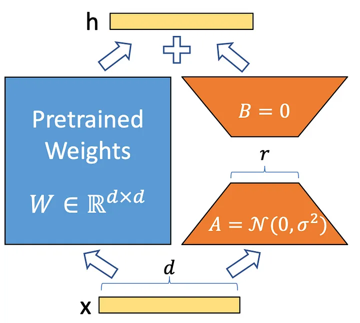
LoRA applies a simple matrix decomposition to each weight matrix update. i.e $\Delta\theta$ ∈ $\Delta W_0$. Considering $\Delta\theta_i$ ∈ $\mathbb{R}^{d x k}$ the update of $i$th weight in network, Lora approx with:
$$ \Delta\theta_i = BA $$
Where, A ∈ $\mathbb{R^{rxd}}$ and B ∈ $\mathbb{R^{dxr}}$ and the rank $r«min(d,k)$. This means that for forward pass of the layer, originally $W x$, is modified to $Wx + BAx$ (as shown in the figure above). Thus instead of learning $d×k$ parameters we now need to learn $(d+k)×r$ which is easily a lot smaller given the multiplicative aspect. A random Gaussian initialization is used for $A$ and $B$ is initially set to 0, so $\Delta\theta_i = BA =0$ at the start of training. The update $\Delta\theta_i or BA$ is additionally scaled with a factor $α/r$ which can be interpreted as a learning rate for the LoRA update.
If we limit the $rank (r)$ to a smaller value in the middle, we can greatly reduce the number of trainable parameters and decrease the dimensionality of the features to $“r « d”$. This will result in an overall parameter count of $"|W|=2×LoRA ×dmodel ×r"$ where, $LoRA$ is the number of $LoRA$ modules used in the entire model
Once the fine-tuning is done, we can just simply update weights in $W$ by adding with its respective $\Delta\theta$.
PyTorch Minimal Implementation
Let’s train a simple implementation of linear regression using PyTorch.
We will create simple training data using $y=\theta X$
Then we will build a LinearRegressionModel to estimate the value of $\theta$. Let’s assume it to be our pre-trained model.
import math
import torch
import torch.nn as nn


# Define dimensions
n = 10000 # Total number of samples
d_in = 1001
d_out = 1000
hidden_dim = 1000

# Moving data to the device
device = torch.device('cuda' if torch.cuda.is_available() else 'cpu')

# Define the data
thetas = torch.randn(d_in, d_out).to(device)

X = torch.randn(n, d_in).to(device)
y = torch.matmul(X, thetas).to(device)

print(f"Shape of X : {X.shape}")
print(f"Shape of y : {y.shape}")
print(f"Shape of θ : {thetas.shape}")
Shape of X : torch.Size([10000, 1001])
Shape of y : torch.Size([10000, 1000])
Shape of θ : torch.Size([1001, 1000])
Now, let’s define our LinearRegressionModel. It consists of two simple linear layers.
class LinearRegressionModel(nn.Module):
    def __init__(self, input_dim, hidden_dim, output_dim):
        super(LinearRegressionModel, self).__init__()
        self.layer1 = nn.Linear(input_dim, hidden_dim, bias=False)

        self.layer2 = nn.Linear(hidden_dim, output_dim,bias=False)

    def forward(self, x):
        out = self.layer1(x)
        out = self.layer2(out)
        return out

def train(model, X, y, batch_size=128, epochs=100):
    opt = torch.optim.Adam(model.parameters())


    for epoch in range(epochs):
        # randomly shuffle the input data
        permutation = torch.randperm(X.size()[0])

        for i in range(0, X.size()[0], batch_size):
            opt.zero_grad()

            indices = permutation[i:i+batch_size]
            batch_x, batch_y = X[indices], y[indices]

            outputs = model(batch_x)
            loss = torch.nn.functional.mse_loss(outputs, batch_y)

            loss.backward()
            opt.step()

        if epoch % 10 == 0:
            with torch.no_grad():
                outputs = model(X)
                loss = torch.nn.functional.mse_loss(outputs, y)
                print(f"Epoch : {epoch }/{epochs} Loss : {loss.item()} ")
# Define the model
model = LinearRegressionModel(d_in, hidden_dim, d_out).to(device)

train(model, X, y)
Epoch : 0/100 Loss : 868.3592529296875
Epoch : 10/100 Loss : 18.999113082885742
Epoch : 20/100 Loss : 1.2845144271850586
Epoch : 30/100 Loss : 0.1564238965511322
Epoch : 40/100 Loss : 0.028503887355327606
Epoch : 50/100 Loss : 0.006223085802048445
Epoch : 60/100 Loss : 0.0016892347484827042
Epoch : 70/100 Loss : 0.7939147353172302
Epoch : 80/100 Loss : 0.2283499538898468
Epoch : 90/100 Loss : 0.2333495020866394
Now that we have our base model that has been pre-trained, let’s assume that we have data from a slightly different distribution
thetas2 = thetas + 1

X2 = torch.randn(n, d_in).to(device)
y2 = torch.matmul(X2, thetas2).to(device)
As we know this data is from a different distribution, if we apply this data to our base model we wont get good result.
loss = torch.nn.functional.mse_loss(model(X2), y2)
print(f"Loss on different distribution: {loss}")
Loss on different distribution: 1013.2288818359375
We now fine-tune our initial model $\theta$. The distribution of the new data is just slighly different from the initial one. It’s just a rotation of the data points, by adding 1 to all thetas. This means that the weight updates are not expected to be complex, and we shouldn’t need a full-rank update in order to get good results.
class LoRAAdapter(nn.Module):
    def __init__(self, model, r=16, alpha=1):
        super(LoRAAdapter, self).__init__()
        self.module_list = nn.ModuleList()
        self.scaling = alpha / r
        self.original_linears = []

        # Go through the layers of the model
        # if the layer is linear layer, add an adpter to it.
        for layer in model.children():
            if isinstance(layer, nn.Linear):
                # Keep a reference to the original linear layers
                # we may need them to add A and B praramters
                self.original_linears.append(layer)

                # Create an adapted layer for each Linear layer
                adapted_layer = AdaptedLinear(layer, r, self.scaling)
                self.module_list.append(adapted_layer)
            else:
                # Keep other types of layers as they are
                self.module_list.append(layer)

    def forward(self, x):
        for layer in self.module_list:
            x = layer(x)
        return x

    def update_original_weights(self):
        with torch.no_grad():
            for adapted_layer, original_layer in zip(self.module_list, self.original_linears):
                delta_theta = torch.matmul(adapted_layer.A, adapted_layer.B) * adapted_layer.scaling
                original_layer.weight.add_(delta_theta.t())


class AdaptedLinear(nn.Module):

    def __init__(self, linear, r, scaling ) -> None:
        super().__init__()
        linear.requires_grad_(False)
        self.linear = linear
        self.A = nn.Parameter(torch.randn(linear.in_features, r))
        self.B = nn.Parameter(torch.zeros(r, linear.out_features))
        self.scaling = scaling

    def forward(self, x):
        return self.linear(x) + torch.matmul(x, torch.matmul(self.A, self.B) * self.scaling)
lora_model = LoRAAdapter(model, r=1).to(device)
We have now initialized our Lora model. For simplicity let’s put $r = 1$. Now, let’s train the model.
train(lora_model,X=X2,y=y2)
Epoch : 0/100 Loss : 1007.549072265625
Epoch : 10/100 Loss : 679.202880859375
Epoch : 20/100 Loss : 317.93316650390625
Epoch : 30/100 Loss : 124.77867889404297
Epoch : 40/100 Loss : 39.598350524902344
Epoch : 50/100 Loss : 9.39522933959961
Epoch : 60/100 Loss : 1.6521010398864746
Epoch : 70/100 Loss : 0.4204731583595276
Epoch : 80/100 Loss : 0.3215165138244629
Epoch : 90/100 Loss : 0.3118535876274109
Up to this point, we just trained the A and B parameters but we still haven’t performed changes in $W x$ i.e. $Wx + BAx$. So the model won’t show any improvements.
loss = torch.nn.functional.mse_loss(model(X2), y2)
print(f"Loss on different distribution: {loss}")
Loss on different distribution: 1013.2288818359375
Now after performing $Wx + BAx$ for each of the linear layers in the model, the loss will converge. i.e We have successfully finetuned our model on new distribution.
lora_model.update_original_weights()
loss = torch.nn.functional.mse_loss(model(X2), y2)
print(f"Loss on different distribution: {loss}")
Loss on different distribution: 0.3048411011695862
Conclusion
To sum it all up: LoRA has two major applications. The first is to finetune large models with low compute, and the second is to adapt large models in a low-data regime.Transformer models are predominantly a smart arrangement of matrix multiplication operations. By applying LoRA exclusively to these layers, the cost of fine-tuning is significantly decreased, yet high performance is still achieved. The experiments detailing this can be found in the LoRA paper.