The Secret Sauce of LLaMA🦙 : A Deep Dive!

Modern Llama. Generated using Stable Diffusion v2

In the information era, a new king reigns supreme: the language model. With the internet drowning in a never-ending flood of data, there is a growing demand for intelligent machines that can not only absorb this data but also produce, analyze, and interact with it in previously unthinkable ways.

Enter LLaMA, Meta’s Large Language Model, a monument to artificial intelligence’s current peak. But what lurks underneath the many layers of this behemoth? How can it understand the complexity of human language and respond with such amazing accuracy? If these questions have ever sparked your interest, you’ve come to the right spot.

A large language model, or LLM, is a digital polyglot that understands and generates human-like language based on huge databases. Consider a computer being that reads nearly every book, article, and paper ever published, embodying humanity’s cumulative knowledge. That is the strength of LLMs. While there are several large models out there, Meta’s LLaMA stands out, pioneering techniques that have revolutionized the field.

This blog will untangle the confusing strings that makeup LLaMa. We will travel through its major components, including ROPE (Rotary Position Embedding), RMSNorm, and SwiGLU, exploring both their theoretical foundations and practical uses. Our journey will not only scratch the surface but also we’ll construct this model from the ground up, guided by the strong PyTorch Lightning’s implementation of LLaMa called lit-llama.

I am utilizing the lit-lama implementation of LLaMa primarily due to its open-source nature, which aligns with the ethos of transparent and accessible development. While it seamlessly integrates with the original LLaMa weights distributed by Meta for research purposes, what sets lit-lama apart is its independent implementation that covers the entire spectrum from pretraining and finetuning to inference. Notably, this entire repo is provided under the Apache 2.0 license, ensuring broad usability and adaptability for a variety of research and development scenarios.

Before we embark on this journey, it’s crucial to have a solid understanding of the Transformer architecture, as i assume you’re well-acquainted with its nuances. You can refer to these blogs to recall the concepts of Transformer.1. 2. 3.

Foundations of LLaMa: A Deeper Dive

1. ROPE(Rotary Position Embedding)

Transformers are widely used models for numerous NLP tasks. However, these models do not naturally comprehend the sequence order (in the context of NLP, the order of words). This is where position embeddings become crucial. Position embeddings identify the position of each token in the sequence. These are incorporated with the token embeddings before being input into the Transformer model, enabling the model to grasp the sequence order.

The majority of methods incorporate position data into token representations by addition operation to include either absolute or relative position information.

$$ \begin{align}\mathbf{q}_m &= \mathbf{W}_q(\mathbf{x}_m + \mathbf{p}_m) \\\mathbf{k}_n &= \mathbf{W}_k(\mathbf{x}_n + \mathbf{p}_n)\\ \mathbf{v}_n &= \mathbf{W}_v(\mathbf{x}_n + \mathbf{p}_n) \\\end{align} $$

This approach has a few drawbacks:

• The vanilla positional encoding is designed for a fixed maximum sequence length. If you have a more extended sequence than the maximum length used during training, handling it becomes problematic. You might need to truncate, split, or find another way to fit it within the maximum length. A model trained with a particular maximum sequence length may not generalize well to sequences of very different lengths, even if they’re within the allowed range. The positional encoding for these lengths might be outside the distribution seen during training.
• The sinusoidal nature of the positional encoding might not always be optimal for capturing very long-term dependencies in long sequences. While self-attention theoretically allows for such connections, in practice, the model might still struggle due to the fixed nature of the encoding.

Why RoPE?

• A key advantage of utilizing rotary embedding is its adaptability. In contrast to position embeddings that are restricted to a certain sequence length, RoPE can be expanded to accommodate any sequence length. This makes RoPE useful for models that must handle text of diverse lengths.
• Rotary embeddings equip linear self-attention with relative position encoding. This implies that models can consider the relative positions of tokens when executing self-attention. This could result in more precise predictions and a deeper understanding of the relationships between tokens.

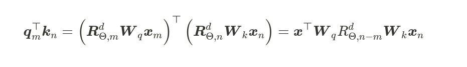
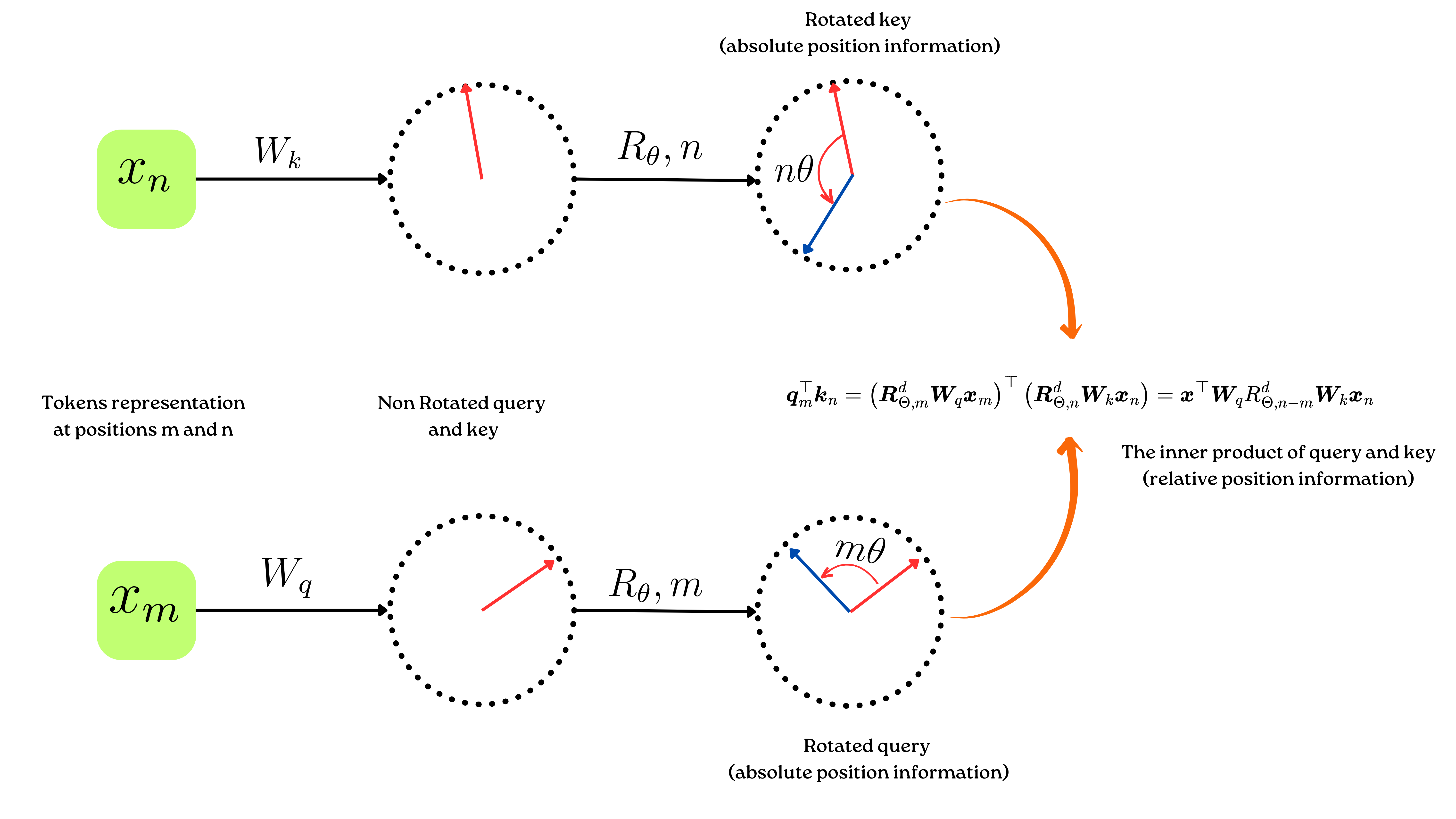
RoPE encodes the absolute position with a rotation matrix and meanwhile incorporates the explicit relative position dependency in the self-attention formulation.

The concept behind the rope is straightforward. Rather than combining the token and position embedding into a single entity by adding them together and calculating q, we should look for transformations for q at m that yield a new vector. Essentially, we rotate the affine-transformed word embedding vector by an amount equivalent to multiples of its position index.

In the original attention, the matrix multiplication between query and key matrices only involves the weight matrices W and the input embedding x.

$$ \begin{aligned} & a_{m, n}=q_m^T k_n=\left[W_q\left(x_m+P E(m)\right)\right]^T W_k\left(x_n+P E(n)\right) \\ \end{aligned} $$

Replace the positional encoding from the vanilla transformer.

$$ \begin{aligned} & a_{m, n}=q_m^T k_n=\left[W_q x_m\right]^T W_k x_n \\\ \end{aligned} $$

Rotate word embedding vector by an amount equivalent to multiples of its position index.

$$ \begin{aligned}& a_{m, n}=q_m^T k_n=\left[R_{\Theta, d}^m\left(W_q x_m\right)\right]^T R_{\Theta, d}^n W_k x_n \\\end{aligned} $$

$$ \begin{aligned}& a_{m, n}=q_m^T k_n=\left(W_q x_m\right)^T R_{\Theta, d}^m{ }^T R_{\Theta, d}^n W_k x_n \\\end{aligned} $$

$$ \begin{aligned}& a_{m, n}=q_m^T k_n=x_m^T W_q^T\left[R_{\Theta, d}^m{ }^T R_{\Theta, d}^n\right] W_k x_n\end{aligned} $$

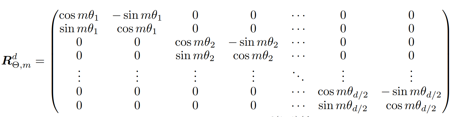
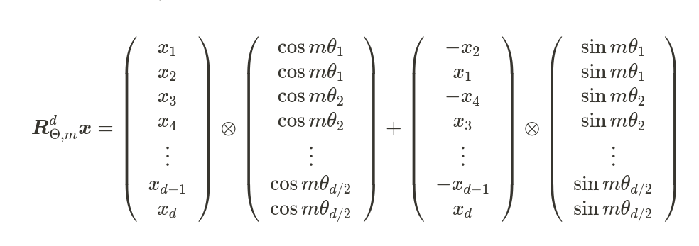
Here, $R_{\Theta, m}^d$ is a rotation matrix. In 2D this matrix is defined as:

$$ R_{\Theta, m}^d=\left(\begin{array}{cc}\cos \left(m \theta_i\right) & -\sin \left(m \theta_i\right) \\sin \left(m \theta_i\right) & \cos \left(m \theta_i\right)\end{array}\right) $$

Where $\theta$ is a nonzero constant. source

The rotation matrix is a function of absolute position. Calculating the inner products of rotated queries and keys results in an attention matrix that is a function of relative position information only.

Attention is relative but how? source

$$ \begin{align}\Big \langle RoPE\big(x^{(1)}_m, x^{(2)}_m, m\big), RoPE\big(x^{(1)}_n, x^{(2)}_n, n\big) \Big \rangle &= \\(x^{(1)}_m \cos m\theta - x^{(2)}_m \sin m \theta)(x^{(1)}_n \cos n\theta - x^{(2)}_n \sin n \theta) &+ \\(x^{(2)}_m \cos m\theta + x^{(1)}_m \sin m \theta)(x^{(2)}_n \cos n\theta + x^{(1)}_n \sin n \theta) &= \\x^{(1)}_m x^{(1)}_n (\cos m\theta \cos n\theta + \sin m \theta \sin n \theta) &+ \\x^{(1)}_m x^{(2)}_n (-\cos m\theta \sin n\theta + \sin m \theta \cos n \theta) &+ \\x^{(2)}_m x^{(1)}_n (-\sin m\theta \cos n\theta + \cos m \theta \sin n \theta) &+ \\x^{(2)}_m x^{(2)}_n (\sin m\theta \sin n\theta + \cos m \theta \cos n \theta) &= \\ x^{(1)}_m x^{(1)}_n \cos (m - n) \theta +x^{(1)}_m x^{(2)}_n \sin(m - n) \theta &+ \\- x^{(2)}_m x^{(1)}_n \sin (m - n) \theta +x^{(2)}_m x^{(1)}_n \cos (m - n) \theta &= \\ \big(x^{(1)}_m \cos (m - n)\theta - x^{(2)}_m \sin (m - n) \theta\big) x^{(1)}_n &+ \\\big(x^{(2)}_m \cos (m - n)m\theta + x^{(1)}_m \sin (m - n) \theta\big) x^{(2)}_n &= \\ \Big \langle RoPE\big(x^{(1)}_m, x^{(2)}_m, m - n\big), RoPE\big(x^{(1)}_n, x^{(2)}_n, 0\big) \Big \rangle \end{align} $$

This shows that for dot-production attention the rotary encoding gives relative attention. so,

Rotary position embedding Overview

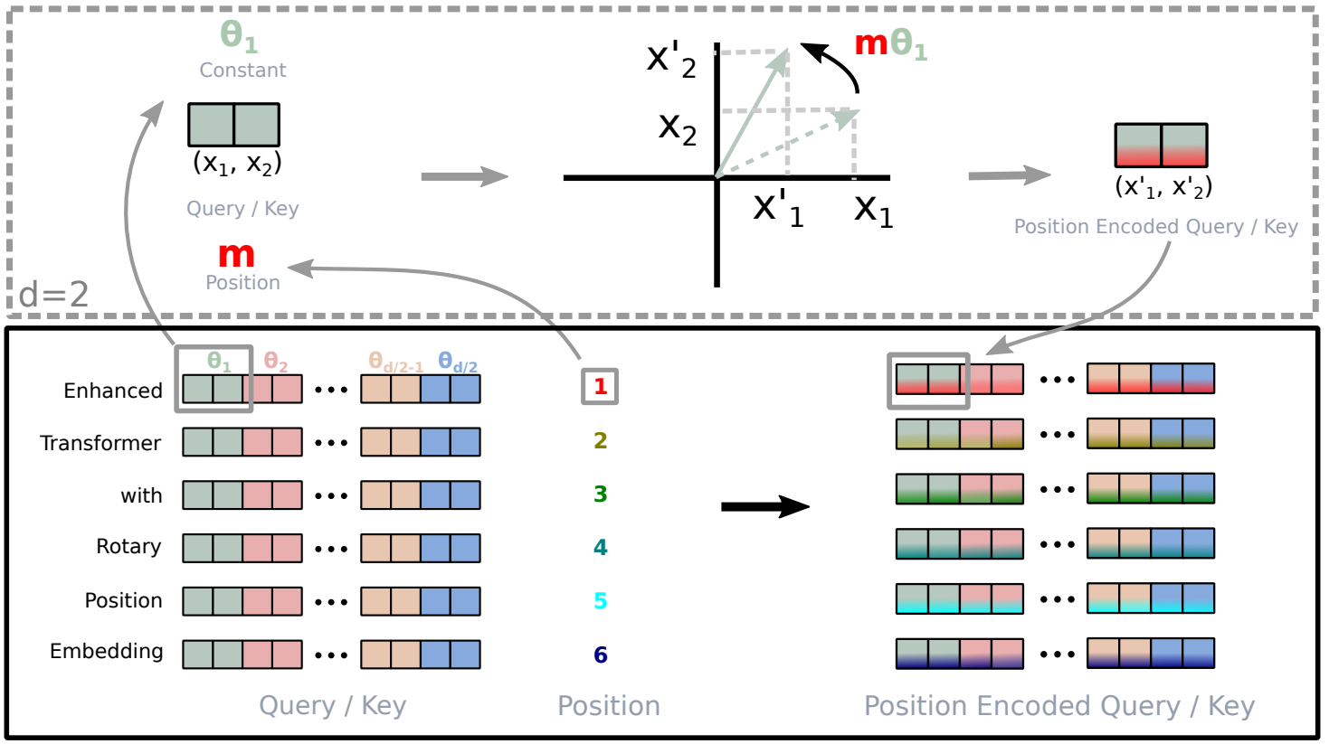
A block-diagonal matrix is a generalization of the 2D rotation matrix to a d-dimensional space. This divides the space into $d/2$ subspace each having different value of $\Theta = {\theta_i = 10000^{-\frac{2(i-1)}{d}}, i \in [1, 2, …, \frac{d}{2}]}$

Apply Rotation to the Queries and Keys:

• Before computing attention scores, the goal is to rotate the query (Q) and key (K) vectors. This rotation is done using the aforementioned sinusoidal values.
• Given a query or key vector $v$ with two parts $v_1$ and $v_2$, the rotated vectors $v’_1$ and $v’_2$ are:

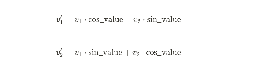
The ${sin_{value}}$ and ${cos_{value}}$ will depend on the position $m$ in the given sequence and the dimension of features.

The following figure illustrates the above concept:

Implementation of Rotary Position Embedding(RoPE) from original paper.Link

Implementation

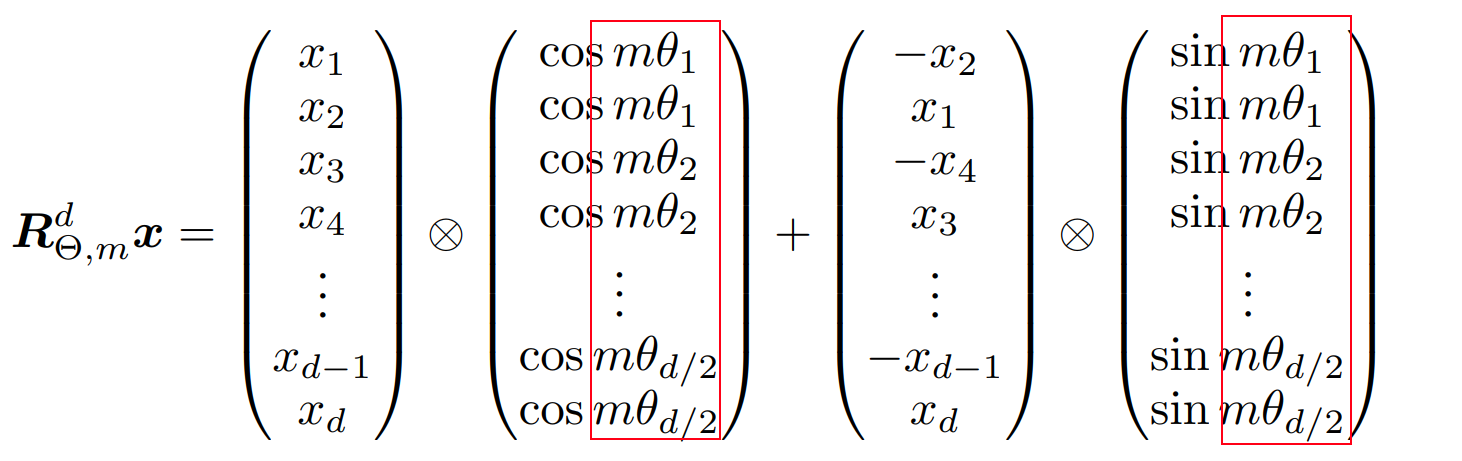
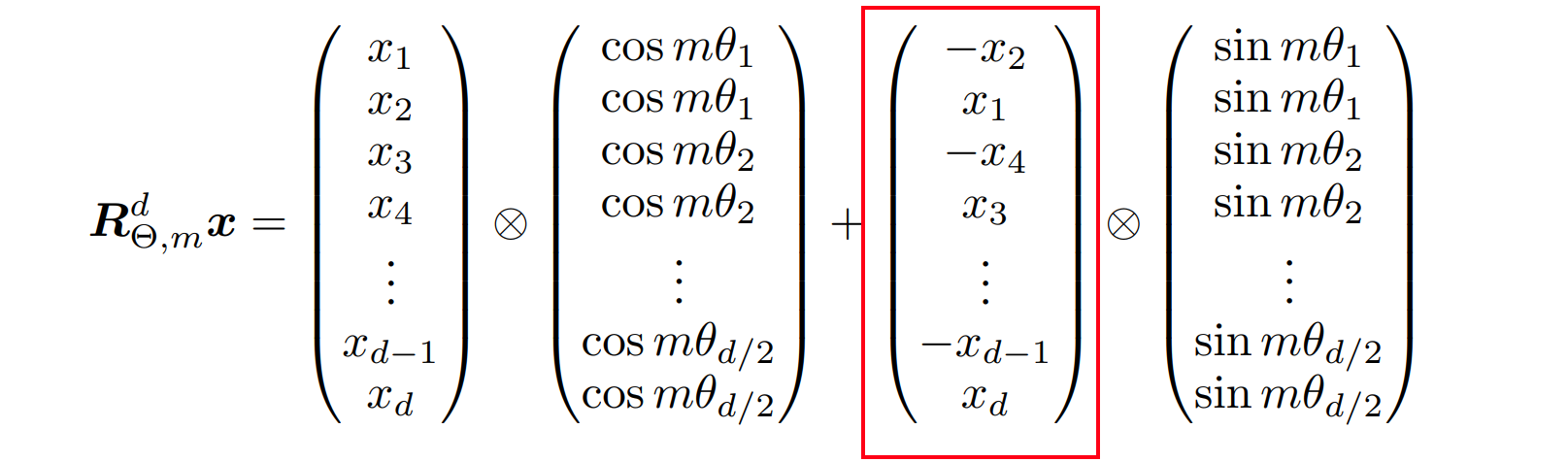
We can see above that ${R}{\Theta, m}^d$ is sparse. A more computationally efficient realization of a multiplication of ${R}{\Theta, m}^d$ and $x \in \mathbb{R}^d$. Where vector $x$ is a query or a key.

As we know that in multi-headed attention, queries and keys are spitted into heads. For each head, we apply the ROPE encodings. Let’s implement ROPE for a single attention head in pure PyTorch.

As we can see from the above equation, the $cos$ and $sin$ values for each head will remain the same, so let’s cache these values.

import torch

def build_cache(dim : int, max_seq_len : int):

    """
    Given a dimension and maximum sequence length, this function returns a tensor 
    containing position encodings obtained by multiplying position indexes with inverse frequencies. 
    The computed encoding is then duplicated along the inverse frequency dimension.

    Parameters:
    - dim (int): Dimensionality for the position encoding, typically the model's hidden dimension size. 
                It determines the number of theta values computed.
    - max_seq_len (int): The maximum sequence length for which to compute position encodings.

    Returns:
    - torch.Tensor: A tensor of shape (max_seq_len, dim) containing the position encodings.

    Examples:
    >>> enc = build_cache(512, 100)
    >>> enc.shape
    torch.Size([100, 512])
    """

    # inverse frequencies [theta_1, theta_2, ..., theta_dim/2]
    inv_freq = 1.0 / (10000 ** (torch.arange(0, dim, 2, dtype=torch.float) / dim))  # -> mθ
    
    # Compute the sequence of position indexes.
    pos = torch.arange(max_seq_len)  # -> m
    
    # Compute the product of the position index and the theta values:
    pos_enc = torch.einsum("n,d->nd", pos, inv_freq) # -> (mθ)
    
    # duplicate each element along inverse frequency dimension
    pos_enc = torch.cat([pos_enc, pos_enc], dim=-1) # -> (mθ,mθ)

    return pos_enc

This build_cache code block will get the product between the position and feature dimension present at that position. We can see this in the following figure:

def negative_half(input_tensor : torch.tensor):

    """
    Applies a specific rotation to the input tensor, often referred to as a "half rotation" 
    in the context of tensor operations.

    Given an input tensor with pairs of elements in its last dimension, this function 
    rotates them such that for each pair (u1, u2), it outputs (-u2, u1). As a result, 
    the sequence [u1, u2, u3, u4, ...] is transformed to [-u2, u1, -u4, u3, ...].

    Parameters:
    - input_tensor (torch.Tensor): The input tensor to be processed. The rotation operation 
                                is applied on the last dimension of this tensor. 

    Returns:
    - torch.Tensor: The rotated tensor with the same shape as the input.

    Examples:
    >>> tensor = torch.tensor([1.0, 2.0, 3.0, 4.0])
    >>> rotated_tensor = negative_half(tensor)
    >>> print(rotated_tensor)
    tensor([-2.,  1., -4.,  3.])
    """

    # Reshaping the tensor so that pairs [u1, u2], [u3, u4], ... are separated
    u =  input_tensor.float().reshape(*input_tensor.shape[:-1], -1, 2)

    # Separating the pairs into two tensors
    u1 = u[..., 0]
    u2 = u[..., 1]
    
    # Reconstructing the tensor after rotation
    u_rotated = torch.stack((-u2, u1), dim=-1)
    
    # Flattening the last two dimensions to get [-u2, u1, -u4, u3, ...]
    u_rotated = u_rotated.view(*u_rotated.shape[:-2], -1)
    
    return u_rotated

The negative_half method will shuffle the elements of $x$ in the second term of the addition is helpful. This method is basically calculating this part:

def rotate(input_tensor : torch.tensor, pos_enc : int):

    """
    Applies a rotation-based position encoding to the input tensor.
    
    The function multiplies the input tensor with the cosine of the position encoding 
    and adds the result of multiplying the negative half of the input tensor with 
    the sine of the position encoding. This is similar to rotating vectors in a 
    complex space using Euler's formula.
    
    Parameters:
    - input_tensor (torch.Tensor): The tensor to which the rotation-based position encoding 
                                  will be applied. It is assumed that the second-to-last 
                                  dimension represents tokens or sequence length.
    - pos_enc (int): Position encoding tensor with values computed elsewhere. The first 
                     dimension of this tensor should be at least as long as the number of 
                     tokens in the `input_tensor`.
                     
    Returns:
    - torch.Tensor: The position-encoded tensor with the same shape as the `input_tensor`.
    
    Examples:
    >>> tensor = torch.tensor([[1.0, 2.0], [3.0, 4.0]])
    >>> pos_enc_tensor = torch.tensor([1.0, 2.0, 3.0])
    >>> rotated_tensor = rotate(tensor, pos_enc_tensor)
    >>> print(rotated_tensor)
    """
    num_tokens = input_tensor.shape[-2]
    pos_enc = pos_enc[:num_tokens]
    return input_tensor * pos_enc.cos() + (negative_half(input_tensor) * pos_enc.sin())

Complete use case:

import torch.nn.functional as F
batch_size = 2
num_heads = 4
seq_len = 16
head_dim = seq_len // num_heads

# random queries and keys
q = torch.randn(batch_size, num_heads, seq_len, head_dim)
k = torch.randn(batch_size, num_heads, seq_len, head_dim)
v = torch.randn(batch_size, num_heads, seq_len, head_dim)

# frequency-encode positions 1 - 512
pos_enc = build_cache(dim=head_dim, max_seq_len=seq_len)

# encode absolute positions into queries and keys
q_rot = rotate(q, pos_enc)
k_rot = rotate(k, pos_enc)

# Step 1: Compute scaled dot-product attention
attn_weights = torch.einsum('bhsd,bhtd->bhst', q_rot, k_rot)  # dot product of queries and keys

# Step 2: Scale the dot products
attn_weights = attn_weights / (head_dim ** 0.5)

# Step 3: Apply softmax to get the weights
attn_weights = F.softmax(attn_weights, dim=-1)

# Step 4: Multiply the weights by the values to get the output
output = torch.einsum('bhst,bhtd->bhsd', attn_weights, v)

print(output.shape)

2. Pre-normalization & RMSNorm

Pre-normalization structure within a transformer block Source

Traditional transformer applies layer normalization after attention and MLP(feed-forward) layer.

LLAMA uses pre-normalization to normalize the input to each transformer sub-layer instead of normalizing the output. The main goal of pre-normalization is to improve the efficiency and stability of the training process by normalizing and reducing variation and correlation of the input features.

In neural networks, the result from the first layer is fed into the second layer, and the result from the second layer is fed into the third, and this process continues. When there are changes in a layer’s parameters, the distribution of inputs for the following layers also changes. This change in distribution is called internal covariate shift.

As per the authors of Batch Normalization :

We define Internal Covariate Shift as the change in the distribution of network activations due to the change in network parameters during training.

This shift can slow down training or cause instability. Normalization helps to stabilize the distributions of layer activations throughout training.

We can mitigate this issue by normalizing the input to the activation functions.

LLAMA uses RMSNorm (Root Mean Square Layer Normalization), an extension of Layer Normalization. RMSNorm is more simpler and efficient than Layer Normalization but achieves similar performance.

RMSNorm

Let’s understand Layer Normalization first:

Layer Normalization for a fully connected layer $i$, neuron $j$ and number of neurons in a layer $m$ :

Calculate mean :

$$ mean_{i}=\frac{1}{m} \sum_{l=1}^{m} \sigma_{i l} $$

Calculate Variance :

$$ var_{i}=\frac{1}{m} \sum_{l=1}^{m}\left(\sigma_{i l}-\text { mean }_{i}\right)^{2} $$

Normalize the feature $j$:

$$ \hat{\sigma}_{i j} = \frac{ \sigma_ij-mean_i}{\sqrt{var_i+\epsilon}} $$

Shift and scale the normalized feature:

Where $\gamma_{i j},\beta_{i,j}$ are learnable parameters. Layer Normalization is successful due to it’s two properties:

1. Re-centering:
   • For each individual data sample, compute the mean of its features.
   • Subtract this mean from each feature of the data sample. This ensures that the features have a mean of zero.
2. Re-scaling:
   • For the same data sample, after re-centering, compute the variance of its features.
   • Normalize each feature by dividing it by the square root of this variance (plus a small epsilon for numerical stability). This ensures that the features have unit variance.
   • After the normalization, the features are typically re-scaled by a learnable parameter and shifted by another learnable parameter. Specifically, if  $\hat{x}$ is the normalized activation, the final output will be $y = \gamma \hat{x} + \beta$, where $\gamma$ and $\beta$ are learnable scaling and shifting parameters, respectively.

The authors of RMSNorm theorize that the key to the success of layer normalization lies in the re-scaling. They suggest RMSNorm, a method that normalizes the input to maintain re-scaling invariance without re-centering the input.

$$  \operatorname{RMS}(\boldsymbol{a})=\sqrt{\frac{1}{n} \sum_{i=1}^{n} a_{i}^{2}} $$

RMSNorm performs at a level similar to LayerNorm, but it reduces the operational time by approximately 10% to 60%.

PyTorch implementation of RMSNorm:

class RMSNorm(nn.Module):

    def __init__(self, input_dim , eps = 1e-6) -> None:
        super().__init__()

        self.g = nn.Parameter(torch.ones(input_dim))
        self.eps = eps

    def forward(self,x):

        # RMS of input
        rms = torch.rsqrt(torch.square(x).mean(dim=-1,keepdim=True) + self.eps)

        # rescaling 
        x  = x * rms

        return x * self.g

3. SwiGLU

SwiGLU is a combination of the Swish activation function and the Gated Linear Unit (GLU) concept. It was introduced in the paper “GLU Variants Improve Transformer” (Sho Takase, Naoaki Okazaki, 2020). The authors propose several variations of the standard GLU that can improve performance on machine translation tasks when used in a Transformer model.

The SwiGLU variant is defined as:

$$ SwiGLU(x, x’) = x ⊙ Swish(x’) $$

where ⊙ is the element-wise multiplication operation, and x’ is the transformed input (generally, a linear transformation of the input x).

Swish

The paper Swish: a Self-Gated Activation Function proposes Swish, also a smooth version of ReLU with a non-zero gradient for negative values.

Swish is a smooth, non-monotonic function that consistently matches or outperforms ReLU.

Simply put, Swish is an extension of the SILU activation function. SILU’s formula $f(x) = x * sigmoid(x)$. The slight modification made in the Swish formulation is the addition of a trainable β parameter, making it $f(x)=xsigmoid(\beta x)$

Swish has several unique characteristics that make it better than ReLU.

• First, Swish is a smooth, continuous function, in contrast to ReLU, which is a piecewise linear function.
• Swish permits a small number of negative weights to pass through, while ReLU sets all negative weights to zero. This property is vital and contributes significantly to the success of non-monotonic smooth activation functions, such as Swish, particularly when used in progressively deeper neural networks. (A non-monotonic function is a type of function that does not consistently increase or decrease in value. In other words, as you move from left to right along the x-axis, a non-monotonic function can either increase or decrease at different points, not following a single direction throughout its domain.)
• The trainable parameter $\beta$ enables the activation function to be fine-tuned more effectively to optimize information propagation and push for smoother gradients.

PyTorch implementation:

import torch
import torch.nn as nn

class Swish(nn.Module):
    def __init__(self, beta: torch.Tensor):
        super().__init__()
        self.beta = nn.Parameter(beta)

    def forward(self, x):
        return x * torch.sigmoid(self.beta * x)

Gated Linear Unit (GLU)

GLU (Gated Linear Units) is a layer within a neural network, rather than a strict activation function. It involves a linear transformation followed by a gating process. This gating process is controlled by a sigmoid function that manages the information flow from the linear transformation.

$$ h_{l}(\mathbf{X})=(\mathbf{X} * \mathbf{W}+\mathbf{b}) \otimes \sigma(\mathbf{X} * \mathbf{V}+\mathbf{c}) $$

$\sigma$ means the sigmoid function. So we have two sets of weights W and V, and two biases, b, and c.

Here is the most intuitive example of GLU I found HERE.

The idea is simple. I want to allow the network to decide how much information should flow through a given path, like a logical gate, hence the name. How?

• If we multiply X by 0, nothing passes.
• If we multiply X by 1, everything passes.
• If we multiply X by 0.5, half of it passes.

It’s inspired by the idea of the gates of LSTMs but applied to convolutions and linear layers, but it’s the same idea.

PyTorch implementation:

class GLU(nn.Module):
    def __init__(self, in_size) -> None:
        super().__init__()

        self.linear1  = nn.Linear(in_size, in_size)
        self.linear2  = nn.Linear(in_size, in_size)

    def forward(self, X):
        return self.linear1(X) * torch.sigmoid(self.linear2(X))

As we now have a clear understanding of the building blocks of SwiGLU, let’s implement it on PyTorch.

import torch
import torch.nn as nn

class Swish(nn.Module):
    def __init__(self, beta: torch.Tensor):
        super().__init__()
        self.beta = nn.Parameter(beta)

    def forward(self, x):
        return x * torch.sigmoid(self.beta * x)

class SwiGLU(nn.Module):
    def __init__(self, in_size, beta: torch.Tensor) -> None:
        super().__init__()

        self.linear1 = nn.Linear(in_size, in_size)
        self.linear2 = nn.Linear(in_size, in_size)
        self.swish = Swish(beta)

    def forward(self, X):
        return self.linear1(X) * self.swish(self.linear2(X))

The LLaMA in PyTorch

The LLaMa architecture is preetry similar to standard transformer architecture with few new adaptations discussed above. The code used below can be found : HERE

Humans learning from LLaMa.Generated using Stable Diffusion 2.0

As mentioned earlier, ill be using a fork of lit-lama repo by Lightning AI. As we have now grasped the fundamental building blocks of LLaMa, let’s get started with the code.

import math
from dataclasses import dataclass
from typing import Optional

import torch
import torch.nn as nn
from torch.nn import functional as F
from typing_extensions import Self

from utils import find_multiple

llama_configs = {
    "7B": dict(n_layer=32, n_head=32, n_embd=4096),
    "13B": dict(n_layer=40, n_head=40, n_embd=5120),
    "30B": dict(n_layer=60, n_head=52, n_embd=6656),
    "65B": dict(n_layer=80, n_head=64, n_embd=8192),
}

These are the different variants of the LLaMa models.

@dataclass
class LLaMAConfig:
    block_size: int = 2048
    vocab_size: int = 32000
    padded_vocab_size: Optional[int] = None
    n_layer: int = 32
    n_head: int = 32
    n_embd: int = 4096

    def __post_init__(self):
        if self.padded_vocab_size is None:
            self.padded_vocab_size = find_multiple(self.vocab_size, 64)

    @classmethod
    def from_name(cls, name: str) -> Self:
        return cls(**llama_configs[name])

The LLaMAConfig class is used to store class variables. Let’s understand each of the class variables:

• block_size : Represents the maximum sequence length the language model can process.
• vocab_size : Represents the size of vocabulary the large language model was trained on.
• n_layer : Represents total number of transformer block.
• n_head : Represents the total number of heads in each transformer block.
• n_embd : Represents the size of embedding.

According to this tweet of Andrej Karpathy, it is important to find the nearest multiple of 64 for your vocab. The tweet explains:

The most dramatic optimization to nanoGPT so far (~25% speedup) is to simply increase vocab size from 50257 to 50304 (nearest multiple of 64). This calculates added useless dimensions but goes down a different kernel path with much higher occupancy. Careful with your Powers of 2.

You can also read more about it HERE.

def __post_init__(self):
    if self.padded_vocab_size is None:
        self.padded_vocab_size = find_multiple(self.vocab_size, 64)

This code block initializes the padded_vocab_size attribute of an object to a multiple of 64 based on the object’s vocab_size, but only if padded_vocab_size is not already set.

class LLaMA(nn.Module):
    def __init__(self, config: LLaMAConfig) -> None:
        super().__init__()
        assert config.padded_vocab_size is not None
        self.config = config

        self.lm_head = nn.Linear(config.n_embd, config.padded_vocab_size, bias=False)
        self.transformer = nn.ModuleDict(
            dict(
                wte=nn.Embedding(config.padded_vocab_size, config.n_embd),
                h=nn.ModuleList([Block(config) for _ in range(config.n_layer)]),
                ln_f=RMSNorm(config.n_embd),
            )
        )

    def _init_weights(self, module: nn.Module) -> None:
        if isinstance(module, nn.Linear):
            torch.nn.init.normal_(module.weight, mean=0.0, std=0.02 / math.sqrt(2 * self.config.n_layer))
        elif isinstance(module, nn.Embedding):
            torch.nn.init.normal_(module.weight, mean=0.0, std=0.02 / math.sqrt(2 * self.config.n_layer))

    def forward(self, idx: torch.Tensor) -> torch.Tensor:
        _, t = idx.size()
        assert (
            t <= self.config.block_size
        ), f"Cannot forward sequence of length {t}, block size is only {self.config.block_size}"

        # forward the LLaMA model itself
        x = self.transformer.wte(idx)  # token embeddings of shape (b, t, n_embd)

        for block in self.transformer.h:
            x = block(x)
        x = self.transformer.ln_f(x)

        logits = self.lm_head(x)  # (b, t, vocab_size)

        return logits

    @classmethod
    def from_name(cls, name: str) -> Self:
        return cls(LLaMAConfig.from_name(name))

The LLaMA model provided is a PyTorch-based implementation. Below is an elaboration on the various components of the code:

1. Initialization:

class LLaMA(nn.Module):
    def __init__(self, config: LLaMAConfig) -> None:
        super().__init__()
        assert config.padded_vocab_size is not None
        self.config = config

Here, the model takes a configuration object, LLaMAConfig, during initialization. An assertion checks that the padded_vocab_size attribute is not None.

1. Model Architecture:

        self.lm_head = nn.Linear(config.n_embd, config.padded_vocab_size, bias=False)
        self.transformer = nn.ModuleDict(
            dict(
                wte=nn.Embedding(config.padded_vocab_size, config.n_embd),
                h=nn.ModuleList([Block(config) for _ in range(config.n_layer)]),
                ln_f=RMSNorm(config.n_embd),
            )
        )

• The lm_head is the final linear layer of the large language model to generate the final prediction. It maps from embeddings to the vocabulary size, which is used for predicting the next word/token. So why are we doing this? This is because we want to represent the probability distribution over the vocabulary to make the prediction.
• transformer is a dictionary of modules, which includes:
  • wte: Word Token Embedding, an embedding layer for the vocabulary. Given tokens, it will generate embeddings of size config.n_embd=4096.
  • h: A list of blocks, with each block being a segment of the transformer architecture. The number of blocks is defined by config.n_layer.
  • ln_f: A final layer normalization, here using RMSNorm.

1. Weight Initialization:

    def _init_weights(self, module: nn.Module) -> None:
        ...

This method initializes the weights of linear and embedding layers based on the model configuration.

1. Forward Pass:

    def forward(self, idx: torch.Tensor) -> torch.Tensor:
        ...

The forward method defines how input data is processed through the model to produce an output. It processes the input tensor, passes it through the transformer blocks, and eventually through the language model head to produce the logits.

Here, idx is the shape of B,T. We haven’t converted the tokens into embedding. _, t = idx.size() : Get the sequence length.

assert (
    t <= self.config.block_size
), f"Cannot forward sequence of length {t}, block size is only {self.config.block_size}"

This will check whether the input sequence is greater than the max sequence length i.e. self.config.block_size.

x = self.transformer.wte(idx) This will convert the input of shape B,T to B,T,n_embd

for block in self.transformer.h:
    x = block(x)
x = self.transformer.ln_f(x)

This passes the embedding throughout n transformer blocks. I think this is the most interesting part of our entire code. We will dive deeper into it next.

As discussed above logits = self.lm_head(x) # (b, t, vocab_size) maps from embeddings to the vocabulary size, which is used for predicting the next word/token.

1. Load Model by Name:

    @classmethod
    def from_name(cls, name: str) -> Self:
        return cls(LLaMAConfig.from_name(name))

This class method allows for creating a LLaMA model instance directly using a name, assuming the LLaMAConfig.from_name(name) can produce the necessary configuration from the provided name.

class Block(nn.Module):
    def __init__(self, config: LLaMAConfig) -> None:
        super().__init__()
        self.rms_1 = RMSNorm(config.n_embd)
        self.attn = CausalSelfAttention(config)
        self.rms_2 = RMSNorm(config.n_embd)
        self.mlp = MLP(config)

    def forward(self, x: torch.Tensor) -> torch.Tensor:
        x = x + self.attn(self.rms_1(x))
        x = x + self.mlp(self.rms_2(x))
        return x

A transformer block typically consists of self-attention mechanisms followed by feed-forward neural networks. The LLaMA model has infused some variations, including the use of RMSNorm for normalization. Forward Pass:

• The input tensor x is first normalized using the first RMSNorm instance.
• Post normalization, it’s fed into the CausalSelfAttention. The result is combined with the original tensor via a residual connection, a vital feature in deep networks for maintaining gradient flow.
• The tensor then undergoes the second RMSNorm normalization.
• The normalized output is processed by the MLP. As before, the resultant is added back to the tensor using a residual connection.
• The processed tensor, rich with information, is then returned.

The Block class crystallizes a singular transformer layer’s operations within LLaMA. With the integral role of RMSNorm already understood, it becomes evident how this block combines normalization, attention, and feed-forward operations to refine the data representation at each layer. When stacked, these blocks work in concert, building upon one another to offer the powerful capabilities of the LLaMA model.

class CausalSelfAttention(nn.Module):
    def __init__(self, config: LLaMAConfig) -> None:
        super().__init__()
        assert config.n_embd % config.n_head == 0

        # key, query, value projections for all heads, but in a batch
        self.c_attn = nn.Linear(config.n_embd, 3 * config.n_embd, bias=False)
        # output projection
        self.c_proj = nn.Linear(config.n_embd, config.n_embd, bias=False)

        self.n_head = config.n_head
        self.n_embd = config.n_embd
        self.block_size = config.block_size
        self.rope_cache: Optional[torch.Tensor] = None

    def forward(self, x: torch.Tensor) -> torch.Tensor:
        B, T, C = x.size()  # batch size, sequence length, embedding dimensionality (n_embd)

        # calculate query, key, values for all heads in batch and move head forward to be the batch dim
        q, k, v = self.c_attn(x).split(self.n_embd, dim=2)

        head_size = C // self.n_head
        k = k.view(B, T, self.n_head, head_size)
        q = q.view(B, T, self.n_head, head_size)
        v = v.view(B, T, self.n_head, head_size)

        if self.rope_cache is None:
            # cache for future forward calls
            self.rope_cache = build_rope_cache(
                seq_len=self.block_size,
                n_elem=self.n_embd // self.n_head,
                dtype=x.dtype,
                device=x.device,
            )

        q = apply_rope(q, self.rope_cache)
        k = apply_rope(k, self.rope_cache)

        k = k.transpose(1, 2)  # (B, nh, T, hs)
        q = q.transpose(1, 2)  # (B, nh, T, hs)
        v = v.transpose(1, 2)  # (B, nh, T, hs)

        # causal self-attention; Self-attend: (B, nh, T, hs) x (B, nh, hs, T) -> (B, nh, T, T)
        #  att = (q @ k.transpose(-2, -1)) * (1.0 / math.sqrt(k.size(-1)))
        #  att = att.masked_fill(self.bias[:,:,:T,:T] == 0, float('-inf'))
        #  att = F.softmax(att, dim=-1)
        #  y = att @ v # (B, nh, T, T) x (B, nh, T, hs) -> (B, nh, T, hs)

        # efficient attention using Flash Attention CUDA kernels
        y = F.scaled_dot_product_attention(q, k, v, attn_mask=None, dropout_p=0.0, is_causal=True)
        y = y.transpose(1, 2).contiguous().view(B, T, C)  # re-assemble all head outputs side by side

        # output projection
        y = self.c_proj(y)

        return y

Here comes the most interesting part of our LLM. Let’s dive into each line of code in detail.

1. Initialization:

• Here, we first ensure that the embedding size (n_embd) is divisible by the number of attention heads (n_head). This is necessary to equally distribute the embeddings across all heads.

• The Key, Query, Value Projections: self.c_attn = nn.Linear(config.n_embd, 3 * config.n_embd, bias=False)

  This transformation is designed to produce key, query, and value tensors, which are essential for the attention mechanism. Normally, you’d expect three separate linear transformations - one for each of key, query, and value. But here, they’re combined into a single transformation for efficiency.

  Input: config.n_embd represents the embedding size of each token in the model. Output: 3 * config.n_embd might look a bit confusing initially, but it makes perfect sense once you understand the purpose. Since we’re generating three different tensors (key, query, and value) and each has an embedding size of config.n_embd, the combined size is 3 * config.n_embd.

1. Forward Pass:

• The input tensor’s dimensions are extracted, where:
  • B represents the batch size.
  • T stands for the sequence length.
  • C denotes the embedding dimensionality.
• The tensor x undergoes the c_attn transformation, splitting the result into query, key, and value tensors (q, k, v).
• These tensors are then reshaped for multi-head attention. Essentially, the embedding dimensionality is divided among the number of attention heads.
• If the rope cache hasn’t been built (i.e., self.rope_cache is None), it’s constructed using the build_rope_cache function. As we already discussed this cache is calculated for a single head and later applied across each head, we can see that n_elem=self.n_embd // self.n_head, this basically means for each token in the sequence, we split the token into n_head, and based on the dimension of the head, we calculate the ROPE cache. This method is pretty much similar to the one we have implemented before. We will discuss some changes in this implementation later. This cache is then applied to the q and k tensors using apply_rope which is also pretty much similar to our previous approach.
• The q, k, and v tensors are transposed to align them for the attention mechanism. Can you tell me why are we performing this transformation? After transposing, we have the final tensor of the shape (B, nh, T, hs). Now if we perform the operation q @ k.t, as the key is transformed, the final tensor will be of shape T,T. This T,T matrix will give us information about, given a token, what’s the relation with other tokens. I think you got an idea of why this transformation is performed. This is done basically to get the attention matrix.
• The main action happens in the causal self-attention mechanism. Normally, one would compute attention scores by multiplying q and k, apply a mask for causality, then use this to weigh the v tensor. Here, however, the mechanism uses the efficient F.scaled_dot_product_attention method, which leverages FlashAttention for faster attention calculations. FlashAttention is a new algorithm to speed up attention and reduce its memory footprint—without any approximation. You can read more about FlashAttention Here, Here, Here.
• The resultant tensor y is reshaped and then undergoes the output projection via the c_proj transformation.

class MLP(nn.Module):
    def __init__(self, config: LLaMAConfig) -> None:
        super().__init__()
        hidden_dim = 4 * config.n_embd
        n_hidden = int(2 * hidden_dim / 3)
        n_hidden = find_multiple(n_hidden, 256)

        self.c_fc1 = nn.Linear(config.n_embd, n_hidden, bias=False)
        self.c_fc2 = nn.Linear(config.n_embd, n_hidden, bias=False)
        self.c_proj = nn.Linear(n_hidden, config.n_embd, bias=False)

    def forward(self, x: torch.Tensor) -> torch.Tensor:
        x = F.silu(self.c_fc1(x)) * self.c_fc2(x)
        x = self.c_proj(x)
        return x

class RMSNorm(nn.Module):
    """Root Mean Square Layer Normalization.

    Derived from <https://github.com/bzhangGo/rmsnorm/blob/master/rmsnorm_torch.py>. BSD 3-Clause License:
    <https://github.com/bzhangGo/rmsnorm/blob/master/LICENSE>.
    """

    def __init__(self, size: int, dim: int = -1, eps: float = 1e-5) -> None:
        super().__init__()
        self.scale = nn.Parameter(torch.ones(size))
        self.eps = eps
        self.dim = dim

    def forward(self, x: torch.Tensor) -> torch.Tensor:
        # NOTE: the original RMSNorm paper implementation is not equivalent
        # norm_x = x.norm(2, dim=self.dim, keepdim=True)
        # rms_x = norm_x * d_x ** (-1. / 2)
        # x_normed = x / (rms_x + self.eps)
        norm_x = torch.mean(x * x, dim=self.dim, keepdim=True)
        x_normed = x * torch.rsqrt(norm_x + self.eps)
        return self.scale * x_normed

def build_rope_cache(seq_len: int, n_elem: int, dtype: torch.dtype, device: torch.device, base: int = 10000) -> torch.Tensor:
    """Enhanced Transformer with Rotary Position Embedding.

    Derived from: <https://github.com/labmlai/annotated_deep_learning_paper_implementations/blob/master/labml_nn/>
    transformers/rope/__init__.py. MIT License:
    <https://github.com/labmlai/annotated_deep_learning_paper_implementations/blob/master/license>.
    """
    # $\\Theta = {\\theta_i = 10000^{\\frac{2(i-1)}{d}}, i \\in [1, 2, ..., \\frac{d}{2}]}$
    theta = 1.0 / (base ** (torch.arange(0, n_elem, 2, dtype=dtype, device=device) / n_elem))

    # Create position indexes `[0, 1, ..., seq_len - 1]`
    seq_idx = torch.arange(seq_len, dtype=dtype, device=device)

    # Calculate the product of position index and $\\theta_i$
    idx_theta = torch.outer(seq_idx, theta).float()

    cache = torch.stack([torch.cos(idx_theta), torch.sin(idx_theta)], dim=-1)

    # this is to mimic the behaviour of complex32, else we will get different results
    if dtype in (torch.float16, torch.bfloat16, torch.int8):
        cache = cache.half()
    return cache

def apply_rope(x: torch.Tensor, rope_cache: torch.Tensor) -> torch.Tensor:
    # truncate to support variable sizes
    T = x.size(1)
    rope_cache = rope_cache[:T]

    # cast because the reference does
    xshaped = x.float().reshape(*x.shape[:-1], -1, 2)
    # uta hami lea cos ra sine lai 2 ota use garinthiyo. Like x_rope, neg_half_x calculate gareko.
    rope_cache = rope_cache.view(1, xshaped.size(1), 1, xshaped.size(3), 2)
    x_out2 = torch.stack(
        [
            xshaped[..., 0] * rope_cache[..., 0] - xshaped[..., 1] * rope_cache[..., 1],
            xshaped[..., 1] * rope_cache[..., 0] + xshaped[..., 0] * rope_cache[..., 1],
        ],
        -1,
    )

    x_out2 = x_out2.flatten(3)
    return x_out2.type_as(x)

The build_rope_cache function is almost identical to build_cache we implemented. Here the cos and sin values are calculated beforehand. Also, build_rope_cache has specific handling for certain data types like torch.float16, torch.bfloat16, and torch.int8, where it casts the computed cache to half precision. build_cache doesn’t handle data types in this manner.

The apply_rope also applies RoPE cache to query and key. But there is a slight difference in how the transformation is applied. I’ll explain what is happening in this method in detail.

We have two tensors: x and rope_cache.

Let’s assume x is a 4D tensor with shape (1, 4, 2, 4) and rope_cache is a 4D tensor with shape (4, 2, 2).

x = tensor([[[[ 0,  1,  2,  3],
          [ 4,  5,  6,  7]],

         [[ 8,  9, 10, 11],
          [12, 13, 14, 15]],

         [[16, 17, 18, 19],
          [20, 21, 22, 23]],

         [[24, 25, 26, 27],
          [28, 29, 30, 31]]]])

Step 1 :

T = x.size(1)

Here, T is simply the size of the second dimension of x, which is 4.

Step 2 :

Next, We resize rope_cache to match the size T:

rope_cache = rope_cache[:T]

This step is redundant because rope_cache already has a size of 4 in its first dimension.

Step 3:

Then, you reshape x to make its last dimension into two parts:

xshaped = x.float().reshape(*x.shape[:-1], -1, 2)

This breaks down as:

1. Convert x into float: x.float()
2. Reshape it: For our tensor, this converts it from shape (1, 4, 2, 4) to (1, 4, 4, 2).

Given the xshaped tensor structure you provided, we can see that its shape is (1, 4, 2, 2, 2). That means you have:

• 1 batch (the outermost dimension)
• 4 channels
• 2x2 spatial dimensions (height x width)
• 2 values for each spatial position (the innermost dimension)

For instance, before reshaping, the first 2x4 matrix in x is:

0,  1,  2,  3
4,  5,  6,  7

After reshaping, the first 4x2 matrix in xshaped would be:

0,  1
2,  3
4,  5
6,  7

Next, you are reshaping the rope_cache:

rope_cache = rope_cache.view(1, xshaped.size(1), 1, xshaped.size(3), 2)

This converts rope_cache from shape (4, 2, 2) to (1, 4, 1, 2, 2). This reshaping is done to align the dimensions of rope_cache with xshaped for broadcasting during the subsequent operations.

Step 3:

Then, you perform element-wise multiplication and subtraction/addition between the reshaped x and rope_cache:

x_out2 = torch.stack(
    [
        xshaped[..., 0] * rope_cache[..., 0] - xshaped[..., 1] * rope_cache[..., 1],
        xshaped[..., 1] * rope_cache[..., 0] + xshaped[..., 0] * rope_cache[..., 1],
    ],
    -1,
)

This is similar to performing rotation using sine and cosine values from rope_cache. The resulting tensor x_out2 has the same shape as xshaped, which is (1, 4, 4, 2). Rotation operation in torch.stack would work element-wise over the tensors. This means that for each position in xshaped, it uses the corresponding position in rope_cache for the rotation calculation.

Breakdown:

Given a 2D rotation matrix:

$$ R(\theta) = \begin{bmatrix} \cos(\theta) & -\sin(\theta) \ \sin(\theta) & \cos(\theta) \end{bmatrix} $$

When you multiply this rotation matrix with a 2D vector $([x, y]^T)$, you get:

$$ R(\theta) \cdot \begin{bmatrix} x \ y \end{bmatrix} = \begin{bmatrix} x\cos(\theta) - y\sin(\theta) \ x\sin(\theta) + y\cos(\theta) \end{bmatrix} $$

Now, let’s connect this to the operations in the code:

• The first component of the output: $x’ = x\cos(\theta) - y\sin(\theta)$ is given by: xshaped[..., 0] * rope_cache[..., 0] - xshaped[..., 1] * rope_cache[..., 1]

Where:

• xshaped[..., 0] corresponds to the x component (or the first value) of our vector.
• xshaped[..., 1] corresponds to the y component (or the second value) of our vector.
• rope_cache[..., 0] is the cosine of the rotation angle.
• rope_cache[..., 1] is the sine of the rotation angle.
• The second component of the output: $y’ = x\sin(\theta) + y\cos(\theta)$ is given by: xshaped[..., 1] * rope_cache[..., 0] + xshaped[..., 0] * rope_cache[..., 1]

The code is essentially applying this rotation to every pair of values in the tensor xshaped using the angles specified in rope_cache.

The torch.stack(..., -1) at the end stacks these computed values along the last dimension. After this operation, for every pair of x and y values in the original xshaped, you have their rotated counterparts stacked together in the resulting tensor.

Inference

For inference, we will be using the pipeline provided by the lit-lama repo. It provides some helpful classes that can potentially speed up the loading and initialization of large models, especially when only parts of the model need to be accessed or when specific tensor initializations are desired. The code also seems to handle some advanced features like quantization and lazy loading of tensors.

let’s break down these classes:

1. EmptyInitOnDevice class:

   This class is a context manager that changes the behavior of tensor initialization to create tensors with uninitialized memory (or “empty tensors”). Additionally, it can set specific devices and data types for tensor initialization and supports specific quantization modes. When this context is active, tensors are initialized without actually assigning them any initial values, making the initialization process faster in some scenarios.

2. NotYetLoadedTensor class:

   Represents a tensor that has not yet been loaded into memory. It is essentially a placeholder that can be transformed into an actual tensor when accessed or used in computations. This class can be especially useful when dealing with large datasets or models, as it allows for lazy loading of data, only loading tensors into memory when they’re actually needed.

3. LazyLoadingUnpickler class:

   Custom unpickler for lazy loading. Pickling is the process of converting a Python object into a byte stream, and unpickling is the reverse operation. The idea here is to load tensors and related objects from the pickled format only when they’re actually accessed or used.

import sys
import time
import warnings
from pathlib import Path
from typing import Optional

import lightning as L
import torch

from tokenizer import  Tokenizer
from utils import EmptyInitOnDevice, lazy_load, llama_model_lookup

@torch.no_grad()
def generate(
    model: torch.nn.Module,
    idx: torch.Tensor,
    max_new_tokens: int,
    max_seq_length: int,
    temperature: float = 1.0,
    top_k: Optional[int] = None,
    eos_id: Optional[int] = None,
) -> torch.Tensor:
    """Takes a conditioning sequence (prompt) as input and continues to generate as many tokens as requested.

    The implementation of this function is modified from A. Karpathy's nanoGPT.

    Args:
        model: The model to use.
        idx: Tensor of shape (T) with indices of the prompt sequence.
        max_new_tokens: The number of new tokens to generate.
        max_seq_length: The maximum sequence length allowed.
        temperature: Scales the predicted logits by 1 / temperature
        top_k: If specified, only sample among the tokens with the k highest probabilities
        eos_id: If specified, stop generating any more token once the <eos> token is triggered
    """
    # create an empty tensor of the expected final shape and fill in the current tokens
    T = idx.size(0)
    T_new = T + max_new_tokens
    empty = torch.empty(T_new, dtype=idx.dtype, device=idx.device)
    empty[:T] = idx
    idx = empty

    # generate max_new_tokens tokens
    for t in range(T, T_new):
        # ignore the not-filled-yet tokens
        idx_cond = idx[:t]
        # if the sequence context is growing too long we must crop it at max_seq_length
        idx_cond = idx_cond if T <= max_seq_length else idx_cond[-max_seq_length:]

        # forward
        logits = model(idx_cond.view(1, -1))
        logits = logits[0, -1] / temperature

        # optionally crop the logits to only the top k options
        if top_k is not None:
            v, _ = torch.topk(logits, min(top_k, logits.size(-1)))
            logits[logits < v[[-1]]] = -float("Inf")

        probs = torch.nn.functional.softmax(logits, dim=-1)
        idx_next = torch.multinomial(probs, num_samples=1)

        # concatenate the new generation
        idx[t] = idx_next

        # if <eos> token is triggered, return the output (stop generation)
        if idx_next == eos_id:
            return idx[:t + 1]  # include the EOS token

    return idx

def main(
    prompt: str = "Hello, my name is",
    *,
    num_samples: int = 1,
    max_new_tokens: int = 50,
    top_k: int = 200,
    temperature: float = 0.8,
    checkpoint_path: Optional[Path] = None,
    tokenizer_path: Optional[Path] = None,
    quantize: Optional[str] = None,
) -> None:
    """Generates text samples based on a pre-trained LLaMA model and tokenizer.

    Args:
        prompt: The prompt string to use for generating the samples.
        num_samples: The number of text samples to generate.
        max_new_tokens: The number of generation steps to take.
        top_k: The number of top most probable tokens to consider in the sampling process.
        temperature: A value controlling the randomness of the sampling process. Higher values result in more random
            samples.
        checkpoint_path: The checkpoint path to load.
        tokenizer_path: The tokenizer path to load.
        quantize: Whether to quantize the model and using which method:
            ``"llm.int8"``: LLM.int8() mode,
            ``"gptq.int4"``: GPTQ 4-bit mode.
    """
    if not checkpoint_path:
        checkpoint_path = Path(f"./checkpoints/lit-llama/7B/lit-llama.pth")
    if not tokenizer_path:
        tokenizer_path = Path("./checkpoints/lit-llama/tokenizer.model")
    assert checkpoint_path.is_file(), checkpoint_path
    assert tokenizer_path.is_file(), tokenizer_path

    fabric = L.Fabric(devices=1)
    dtype = torch.bfloat16 if fabric.device.type == "cuda" and torch.cuda.is_bf16_supported() else torch.float32

    print("Loading model ...", file=sys.stderr)
    t0 = time.time()
    with lazy_load(checkpoint_path) as checkpoint:
        name = llama_model_lookup(checkpoint)

        with EmptyInitOnDevice(
                device=fabric.device, dtype=dtype, quantization_mode=quantize
        ):
            model = LLaMA.from_name(name)

        model.load_state_dict(checkpoint)
    print(f"Time to load model: {time.time() - t0:.02f} seconds.", file=sys.stderr)

    model.eval()
    model = fabric.setup_module(model)

    tokenizer = Tokenizer(tokenizer_path)
    encoded_prompt = tokenizer.encode(prompt, bos=True, eos=False, device=fabric.device)

    L.seed_everything(1234)
    for i in range(num_samples):
        t0 = time.perf_counter()
        y = generate(
            model,
            encoded_prompt,
            max_new_tokens,
            model.config.block_size,  # type: ignore[union-attr,arg-type]
            temperature=temperature,
            top_k=top_k,
        )
        t = time.perf_counter() - t0
        print('\\n\\n')
        print(tokenizer.decode(y))
        print('\\n\\n')
        print(f"Time for inference {i + 1}: {t:.02f} sec total, {max_new_tokens / t:.02f} tokens/sec", file=sys.stderr)
    if fabric.device.type == "cuda":
        print(f"Memory used: {torch.cuda.max_memory_reserved() / 1e9:.02f} GB", file=sys.stderr)

main("Artificial Intelligence is the")

Loading model ...
Time to load model: 17.45 seconds.
You are using a CUDA device ('NVIDIA GeForce RTX 3090') that has Tensor Cores. To properly utilize them, you should set `torch.set_float32_matmul_precision('medium' | 'high')` which will trade-off precision for performance. For more details, read <https://pytorch.org/docs/stable/generated/torch.set_float32_matmul_precision.html#torch.set_float32_matmul_precision>
Global seed set to 1234

Artificial Intelligence is the ability of a computer to imitate intelligent behaviour without being programmed, such as learning in a self-directed way to do a specific task, and then not just repeating the task, but improving itself. This is different from Traditional Artificial Intelligence which is any

Time for inference 1: 1.41 sec total, 35.55 tokens/sec
Memory used: 13.52 GB

References

LLaMa

• Original Paper : https://arxiv.org/abs/2302.13971
• https://akgeni.medium.com/llama-concepts-explained-summary-a87f0bd61964
• https://kikaben.com/llama-2023-02/
• https://cameronrwolfe.substack.com/p/llama-llms-for-everyone
• https://vinija.ai/models/LLaMA/

Implementation code

• https://github.com/Lightning-AI/lit-llama

ROPE

• Original Paper : https://arxiv.org/pdf/2104.09864.pdf
• https://blog.eleuther.ai/rotary-embeddings/
• https://nn.labml.ai/transformers/rope/index.html#:~:text=This%20is%20an%20implementation%20of,incorporates%20explicit%20relative%20position%20dependency.
• https://serp.ai/rotary-position-embedding/
• https://medium.com/@andrew_johnson_4/understanding-rotary-position-embedding-a-key-concept-in-transformer-models-5275c6bda6d0
• https://github.com/lucidrains/rotary-embedding-torch
• http://krasserm.github.io/2022/12/13/rotary-position-embedding/

YouTube

• https://youtu.be/YMcwsLGU_U8
• https://youtu.be/GQPOtyITy54

Swish

• https://blog.paperspace.com/swish-activation-function/#:~:text=Simply%20put,%20Swish%20is%20an,Function%20Approximation%20in%20Reinforcement%20Learning%22
• https://medium.com/@neuralnets/swish-activation-function-by-google-53e1ea86f820#:~:text=Swish%20is%20a%20smooth,%20non,that%20actually%20creates%20the%20difference

GLU

• https://medium.com/deeplearningmadeeasy/glu-gated-linear-unit-21e71cd52081

RMSNorm

• https://akgeni.medium.com/llama-concepts-explained-summary-a87f0bd61964
• https://kikaben.com/llama-2023-02/