|
|---|
| Image by Martin Adams |
In this Transformers Optimization series, we will explore various optimization techniques for Transformer models. As a kickoff piece, we will dive deep into KV Cache, an inference optimization technique to significantly enhance the inference performance of large language models.
What is KV Cache?
A common technique for improving the performance of large model inferences is by using the KV cache of the last inference. Using the KV cache of the last inference improves inference performance and reduces end-to-end latency without affecting any accuracy.
Why KV Cache?
While generating text (tokens) in autoregressive language models like GPT, all the previously generated tokens are fed into the network when generating a new token. Here, the hidden representation of the previously generated tokens needs to be recalculated each time a new token is generated. This causes a lot of computational waste. Let’s take an example:
import torch

import torch
from transformers import AutoTokenizer, AutoModelForCausalLM
# torch.manual_seed(0)

class Sampler:
    def __init__(self , model_name : str ='gpt2-medium') -> None:

        self.device = 'cuda' if torch.cuda.is_available() else 'cpu'
        self.tokenizer = AutoTokenizer.from_pretrained(model_name)
        self.model = AutoModelForCausalLM.from_pretrained(model_name).to("cpu").to(self.device)

    def encode(self, text):
        return self.tokenizer.encode(text, return_tensors='pt').to(self.device)

    def decode(self, ids):
        return self.tokenizer.decode(ids)

    def get_next_token_prob(self, input_ids: torch.Tensor):
        with torch.no_grad():
            logits = self.model(input_ids=input_ids).logits
        logits = logits[0, -1, :]
        return logits

class GreedySampler(Sampler):
    def __call__(self, prompt, max_new_tokens=10):
        predictions = []
        result = prompt
        # generate until max_len
        for i in range(max_new_tokens):

            print(f"step {i} input: {result}")
            input_ids = self.encode(result)
            next_token_probs = self.get_next_token_prob(input_ids=input_ids)

            # choose the token with the highest probability
            id = torch.argmax(next_token_probs, dim=-1).item()
            # convert to token and add new token to text
            result += self.decode(id)

            predictions.append(next_token_probs[id].item())

        return result
gs = GreedySampler()
gs(prompt="Large language models are recent advances in deep learning", max_new_tokens=10)

step 0 input: Large language models are recent advances in deep learning
step 1 input: Large language models are recent advances in deep learning,
step 2 input: Large language models are recent advances in deep learning, which
step 3 input: Large language models are recent advances in deep learning, which uses
step 4 input: Large language models are recent advances in deep learning, which uses deep
step 5 input: Large language models are recent advances in deep learning, which uses deep neural
step 6 input: Large language models are recent advances in deep learning, which uses deep neural networks
step 7 input: Large language models are recent advances in deep learning, which uses deep neural networks to
step 8 input: Large language models are recent advances in deep learning, which uses deep neural networks to learn
step 9 input: Large language models are recent advances in deep learning, which uses deep neural networks to learn to
Can you see the problem here? As the input tokens for each inference process become longer, it increases inference FLOPs (floating point operations). KV cache solves this problem by storing hidden representations of previously computed key-value pairs while generating a new token.
Let’s take an example of step 4. Here, for generating the word deep, we feed only the uses word into the model and fetch the representation of Large language models are recent advances in deep learning, which from the cache.
Working of KV cache:
Suppose we have n transformer layers in the architecture. Then each of the heads will maintain its own separate KV cache:
class SelfAttention(nn.Module):
    def __init__(self, args: ModelArgs):
        super().__init__()

        ...

        self.cache_k = torch.zeros((args.max_batch_size, args.max_seq_len, self.n_kv_heads, self.head_dim))
        self.cache_v = torch.zeros((args.max_batch_size, args.max_seq_len, self.n_kv_heads, self.head_dim))
During the forward propagation, the cache will be prefilled and accessed as follows:
    def forward(
        self,
        x: torch.Tensor,
        start_pos: int,
        freqs_complex: torch.Tensor
    ):
        ...

        # Input shape : (B, 1, Dim)
        # xk of shape (B, 1, H_KV, Head_Dim)
        # xv of shape (B, 1, H_KV, Head_Dim)
        # Replace the entry in the cache
        self.cache_k[:batch_size, start_pos : start_pos + seq_len] = xk
        self.cache_v[:batch_size, start_pos : start_pos + seq_len] = xv

        # (B, Seq_Len_KV, H_KV, Head_Dim)
        keys = self.cache_k[:batch_size, : start_pos + seq_len]
        # (B, Seq_Len_KV, H_KV, Head_Dim)
        values = self.cache_v[:batch_size, : start_pos + seq_len]
Mathematically Given that the generated token is at $i^{th}$ the transformer layer. It is expressed as the following $t^{i} \in \mathbb{R} ^ {b \times 1 \times h}$. The calculations inside the $i^{th}$ transformer are divided into two parts: updating the KV cache and calculating the $t^{i+1}$.
$$ \begin{array}{l}x_{K}^{i} \leftarrow \operatorname{Concat}\left(x_{K}^{i}, t^{i} \cdot W_{K}^{i}\right) \\ x_{V}^{i} \leftarrow \operatorname{Concat}\left(x_{V}^{i}, t^{i} \cdot W_{V}^{i}\right)\end{array} $$
Now the remaining calculation: $$ \begin{array}{c}t_{Q}^{i}=t_{i} \cdot W_{Q}^{i} \\ t_{\text {out }}^{i}=\operatorname{softmax}\left(\frac{t_{Q}^{i} x_{K}^{i^{T}}}{\sqrt{h}}\right) \cdot x_{V}^{i} \cdot W_{O}^{i}+t^{i} \\ t^{i+1}=f_{\text {activation}}\left(t_{\text {out }}^{i} \cdot W_{1}\right) \cdot W_{2}+t_{\text {out }}^{i}\end{array} $$
To get a better understanding of the steps above, let’s have a look at a visual representation of KV Cache.
Consider a transformer architecture with 12 attention heads and KV Cache. The following figure represents the transformer state while generating $9th$ token of the input sequence.
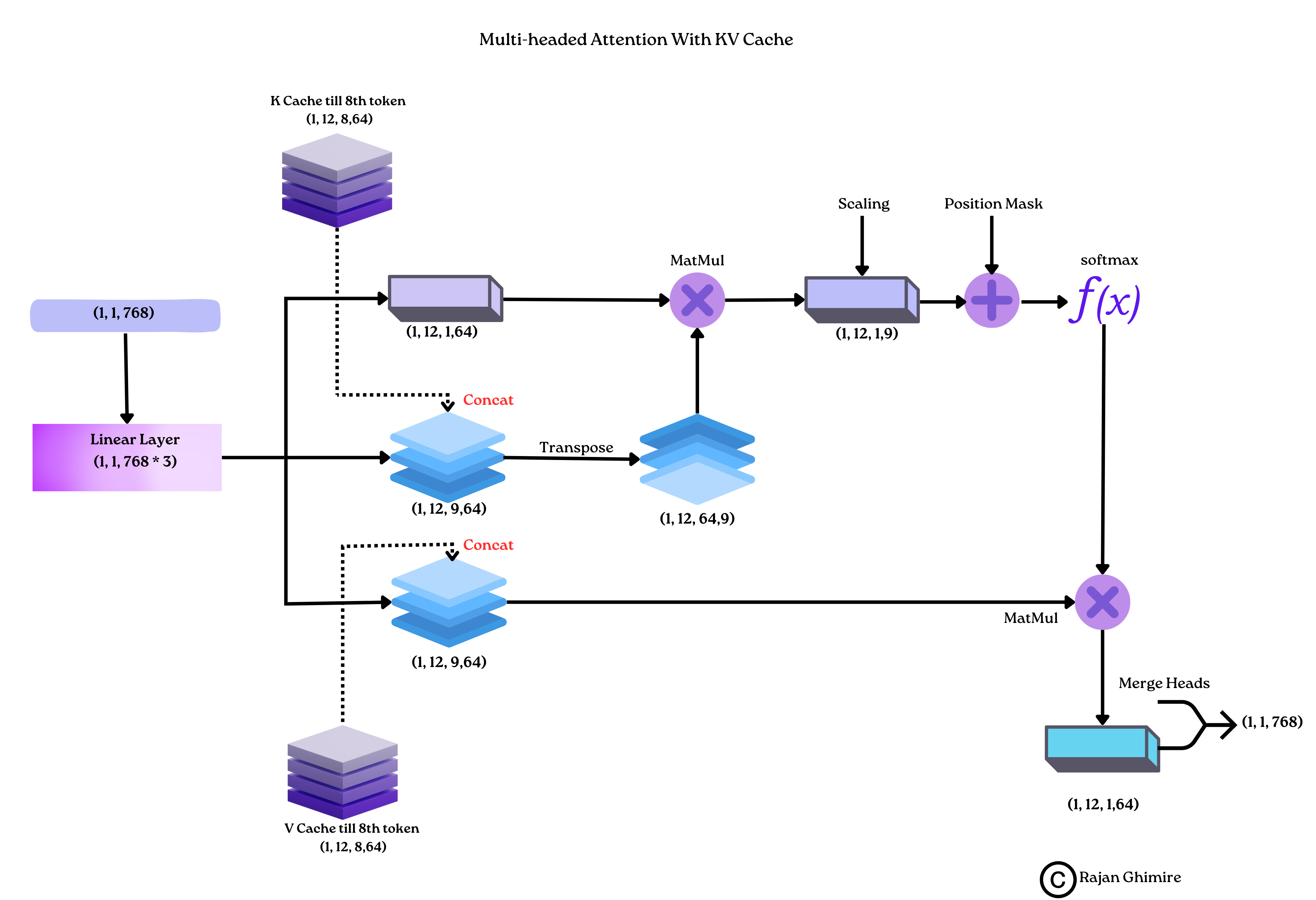
|
|---|
| KV cahce working. |
FLOPs comparison of vanilla Transformer and Transformer with KV Cache.
FLOPs, floating point operations, represent the number of floating-point number operations, measuring the amount of computation.
Calculating FLOPs for Matrix Multiplication:
Let $A \in R^{1 \times n}, B \in R^{n \times 1}$, to compute $AB$ we need $n$ multiplication operations and $n$ addition operations. Then total FLOPs is $2n$. Also, if $A \in R^{m \times n}, B \in R^{n \times p}$ then, to compute $AB$ the number of floating-point arithmetic required is $2mnp$.
Basic Notations:
$b$ = Batch Size
$s$ = Sequence Length
$h$ = Hidden Dimension
$x$ = input
$num\_head$ = Total number of heads
$head\_dim$ = Hidden Dimension of each head.
In self-attention block :
Step 1:
$$ Q = x W_q \ K = x W_k \ V = x W_v $$
Input $x$ of shape = $(b,s,h)$. Shape of weights = $(h,h)$
$$ (b,s,h) (h,h) \rightarrow (b,s,h) $$ Total Computations: $2bsh^2$. For Q, K, V its $3 \times 2bsh^2 \rightarrow 6bsh^2$
Step 2: For attention calculation :
$$ x_{\text {out }}=\operatorname{softmax}\left(\frac{Q K^{T}}{\sqrt{h}}\right) \cdot V \cdot W_{o}+x $$
Step 2.1: For $QK^T$
$$ (b,num\_head,s,head\_dim) \times (b,num\_head,head\_dim, s) \rightarrow (b,num\_headk,s,s) $$ So, the total computations is $2bs^2h$.
Step 2.2 For $\operatorname{softmax}\left(\frac{Q K^{T}}{\sqrt{h}}\right) \cdot V$
$$ (b,num\_head,s,s) \times (b,num\_head,s,head\_dim) \rightarrow (b,num\_head,s,head\_dim) $$ The total claculation is $2bs^2h$.
2.3 For linear layer after attention: (for $W_o$) $$ (b,s,h) (h,h) \rightarrow (b,s,h) $$ Total Computations: $2bh^2$.
Step 3: For MLP block $$ x=f_{\text {activation }}\left(x_{\text {out }} W_{1}\right) W_{2}+x_{\text {out }} $$
Step 3.1: For the first linear layer, the input and output shapes of matrix multiplication are $$ (b, s, h) \times(h, 4 h) \rightarrow(b, s, 4 h) $$ Total Computations: $8bsh^2$. Step 3.2: For the second linear layer, the input and output shapes of matrix multiplication are $$ [b, s, 4 h] \times[4 h, h] \rightarrow[b, s, h] $$ Total Computations: $8bsh^2$.
Step 4: For hidden layer to Vocabulary mapping layer
$$ (b, s, h) \times(h, V) \rightarrow(b, s, V) $$ Total Computations : $2bshV$.
Therefore, total amount of computation for transformer is : $\left(24 b s h^{2}+4 b s^{2} h\right)+2 b s h V$
If we have $n$ transformer layers then, total number of computation will be $$ n \times \left(24 b s h^{2}+4 b s^{2} h\right)+2 b s h V $$
Flops in Transformers with KV cache
As we know, for each iteration, we will be passing a single token, so the input will be of shape: $(b,1,h)$. Step 1: $$ Q = x W_q \ K = x W_k \ V = x W_v $$ Input $x$ of shape = $(b,s,h)$. Shape of weights = $(h,h)$
$$ (b,1,h) (h,h) \rightarrow (b,1,h) $$ Total calculations: $2bsh^2$. For Q, K, V its $3 \times 2bsh^2 \rightarrow 6bh^2$
Step 2: For attention calculation.
$$ x_{\text {out }}=\operatorname{softmax}\left(\frac{Q K^{T}}{\sqrt{h}}\right) \cdot V \cdot W_{o}+x $$
Step 2.1: For $QK^T$
$$ (b,num\_head,1,head\_dim) \times (b,num\_head,head\_dim, KV\_Length + s) \rightarrow (b,num\_head,1,KV\_Length + 1) $$ So, the total computations is $2bs(KV\_Length + 1)h$.
Step 2.2 For $\operatorname{softmax}\left(\frac{Q K^{T}}{\sqrt{h}}\right) \cdot V$
$$ (b,num\_head,1,KV\_Length + 1) \times (b,num\_head,KV\_Length + 1,head\_dim) \rightarrow (b,num\_head,1,head\_dim) $$ The total claculation is $2bs(KV\_Length + 1)h$.
2.3 For linear layer after attention: (for $W_o$) $$ (b,1,h) (h,h) \rightarrow (b,1,h) $$ Total calculations: $2bh^2$.
Step 3: For MLP block $$ x=f_{\text {gelu }}\left(x_{\text {out }} W_{1}\right) W_{2}+x_{\text {out }} $$
3.1 For the first linear layer, the input and output shapes of matrix multiplication are $$ (b, 1, h) \times(h, 4 h) \rightarrow(b, 1, 4 h) $$ Total Computations: $8bh^2$. 3.2 For the second linear layer, the input and output shapes of matrix multiplication are $$ [b, 1, 4 h] \times[4 h, h] \rightarrow[b, 1, h] $$ Total Computations: $8bh^2$.
Step 4: For hidden layer to Vocabulary mapping layer
$$ (b, 1, h) \times(h, V) \rightarrow(b, 1, V) $$ Total Computations : $2bhV$.
Therefore, the total amount of computation for the KV-transformer is: $24 b h^{2}+4 b h+4 b(KV\_Length) + 2bhV h$
If we have $n$ transformer layers then, total number of computation will be $$ n \times (24 b h^{2}+4 b h+4 b(KV\_Length)) + 2bhV h $$
Conclusion
If we have a sufficiently long sequence length $s$, then floating point operations in the KV transformer will be significantly less than those in the vanilla one.
If : $$ F_{\text{Vanilla}}(n, b, s, h, V) = n \times (24 b s h^{2}+4 b s^{2} h) + 2 b s h V \\ F_{\text{KV}}(n, b, h, KV\_Length, V) = n \times (24 b h^{2}+4 b h+4 b KV\_Length) + 2 b h V \ $$
Then :
$$ \lim_{{s \to \infty}} F_{\text{Vanilla}}(n, b, s, h, V) > \lim_{{s \to \infty}} F_{\text{KV}}(n, b, h, KV\_Length, V) $$
References
- https://browse.arxiv.org/pdf/2211.05102.pdf
- https://kipp.ly/transformer-inference-arithmetic/
- https://www.dipkumar.dev/becoming-the-unbeatable/posts/gpt-kvcache/
- https://www.youtube.com/watch?v=80bIUggRJf4
- https://www.youtube.com/watch?v=80bIUggRJf4
- https://www.youtube.com/watch?v=IGu7ivuy1Ag
- https://zhuanlan.zhihu.com/p/630832593
- https://zhuanlan.zhihu.com/p/633653755
- https://zhuanlan.zhihu.com/p/624740065